Describing a model with an R formula

Formulas in R

Graphical examples of formulas

AUTHOR

AFFILIATION

Jon Yearsley

School of Biology and Environmental Science, UCD

How to Read this Tutorial

This tutorial is a mixture of R code chunks and explanations of the code. The R code chunks will appear in boxes.

Below is an example of a chunk of R code:

# This is a chunk of R code. All text after a # symbol is a comment
# Set working directory using setwd() function
setwd('Enter the path to my working directory')

# Clear all variables in R's memory
rm(list=ls())    # Standard code to clear R's memory

Sometimes the output from running this R code will be displayed after the chunk of code.

Here is a chunk of code followed by the R output

2 + 4            # Use R to add two numbers

[1] 6

Introduction

This worksheet gives examples of how R uses formulas to specify a general linear model. We’ve divided up the examples to correspond to classical analyses of:

ANOVA (analysis of variance): continuous response variable, categorical explanatory variables
linear regression: continuous response variable, continuous explanatory variables
ANCOVA (analysis of covariance): continuous response variable, continuous and categorical explanatory variables

In R these models could be fitted to data using thelm()function.

Thelm()function fits the models using a method called maximum likelihood. Maximum likelihood methodology is a development upon the classical methods (such as least-squares fits) and is currently the most common method of fitting models to data.

Description of the variables

All the variables used in the examples come from a set of human volunteers who were taking part in a scientific study.

Variable	Description
HEIGHT	The height (m) of a human. This variable is the response variable in all the models. It is aquantitative, continuous variable.
WEIGHT	The weight (kg) of a human. This variable is used as an explanatory variable in some of the examples. It is aquantitative, continuous variable.
SEX	The sex of a human volunteer. This variable is used as an explanatory variable in some of the examples. It is aqualitative variable(commonly called afactor).
GROUP	The human volunteers were divided into two groups (A, B). This variable records the group each volunteer was assigned to. This variable is used as an explanatory variable in some of the examples. It is aqualitative variable(commonly called afactor).
SUBGROUP	The human volunteers were further divided into four subgroups (G1, G2, G3, G4) that isnested within GROUP(G1 and G2 within group A, G3 and G4 within group B). This variable records the subgroup each volunteer was assigned to. This variable is used as an explanatory variable in some of the examples. It is aqualitative variable(commonly called afactor).

ANOVA model formulas

R formula	Description	Graphical description
`HEIGHT ~ 1`	Fits a normal distribution with a single mean and standard deviation for the heights of people in one population.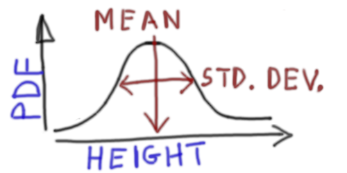
.	Representing the above model by just the mean and standard deviation gives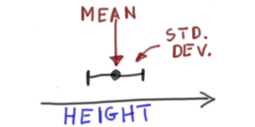
`HEIGHT ~ 1 + SEX`	Fits two normal distributions (one for males and one for females) with different mean heights and the same standard deviation (standard deviation is the same for males and females)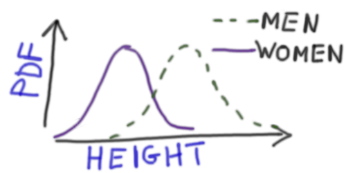
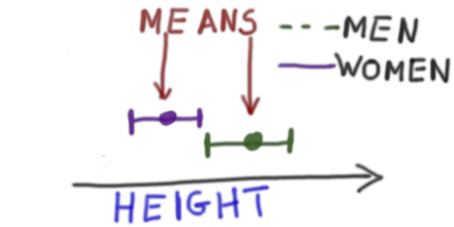
`HEIGHT ~ SEX`	Same as above (the`1`will be added by R automatically). The image on the right just shows means and standard deviation instead of the entire distribution.

Two explanatory variables (nested)

In the example below all factors are fixed butSUBGROUPis nested withinGROUP. Notice that there is no main effect ofSUBGROUPbecause of the nesting.

R formula	Description	Graphical description
`HEIGHT ~ SEX + GROUP +GROUP:SUBGROUP`	Fits five mean heights (males and females in two groups with each group divided into two sub-groups) and single standard deviation (assumed the same for males and females in all groups and sub-groups). The image on the right just shows means and standard deviation instead of the entire distribution.
`HEIGHT ~ SEX + GROUP +SUBGROUP %in% GROUP`	Same as above.

Two explanatory variables (not-nested)

R formula	Description	Graphical description
`HEIGHT ~ SEX + GROUP +SEX:GROUP`	Fits four mean heights (males and females in two groups) and a single standard deviation (assumed the same for males and females in all groups). The image on the right just shows means and standard deviation instead of the entire distribution.
`HEIGHT ~ SEX*GROUP`	Same as above. R interprets`A*B = A+B+A:B`.
`HEIGHT ~ SEX + GROUP`	Fits three mean heights (the interaction term A:B is missing, implying that the mean height differences between men and women is the same in all groups) and a single standard deviation (assumed the same for males and females in all groups)

Linear regression model formulas

R formula	Description	Graphical description
`HEIGHT ~ 1 + WEIGHT`	Fits a straight line relationship (intercept and slope) between peoples HEIGHT and WEIGHT. The mathematical relationship is $HEIGHT = a + b WEIGHT$ where $a$ = intercept, $b$ =slope. The image on the right shows only the mean. For clarity, random variation around the line is not shown.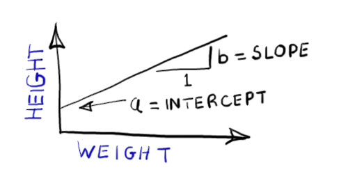
`HEIGHT ~ WEIGHT`	Same as above (R will add an intercept by default)
`HEIGHT ~ 0 + WEIGHT`	As above, but forces the line to pass through the origin (intercept=0, meaning when WEIGHT=0 then HEIGHT=0). The mathematical relationship is $HEIGHT = b WEIGHT$ where $b$ =slope. The image on the right shows only the mean. For clarity, random variation around the line is not shown.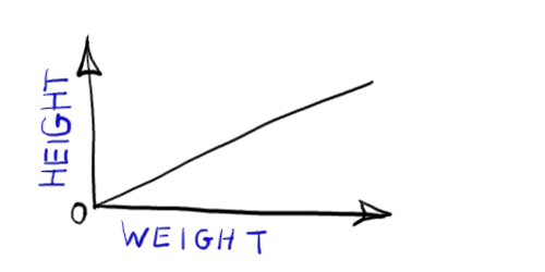

ANCOVA model formulas

R formula	Description	Graphical description
`HEIGHT ~ SEX*WEIGHT`	Fits two straight line relationships (two intercepts and two slopes) between people’s HEIGHT and WEIGHT. One line is the height-weight relationship for men, the other line is the relationship for women. The image on the right shows only the mean. For clarity, random variation around the line is not shown.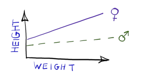
`HEIGHT ~ SEX + SEX:WEIGHT`	Same as the above.
`HEIGHT ~ SEX + WEIGHT`	Fits two straight line relationships with the same slope but different intercepts. Only the intercept can differ between men and women. The image on the right shows only the mean. For clarity, random variation around the line is not shown.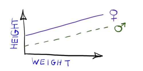
`HEIGHT ~ 1 + SEX:WEIGHT`	Fits two straight line relationships with the same intercept but different slopes. Only the slope can differ between men and women. The image on the right shows only the mean. For clarity, random variation around the line is not shown.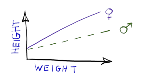
`HEIGHT ~ 0 + SEX:WEIGHT`	Fits two straight line relationships with different slopes, forcing the intercept to be the origin. The image on the right shows only the mean. For clarity, random variation around the line is not shown.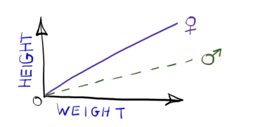

Worked examples

We now show some examples of using these models and fitting them by maximum likelihood (usinglm()) to a real data. Remember,lm()assumes that the random error that cannot be explained by the model (theresiduals) always have a normal distribution with a single well defined spread (the standard deviation $σ$ ).

$RESPONSE_{i} = EXPLANATORY MODEL_{i} + ERROR_{i}$

The i subscript represent the i^thobservation, and remind us that each observation is “explained” by the explanatory model and a random error (the normal distribution).

We have a data frame (called heights) containing the data. Here is a summary of the data

 GROUP    SUBGROUP      SEX           HEIGHT          WEIGHT      
 A:2054   G1:1065   Female:1552   Min.   :1.409   Min.   : 35.80  
 B:2702   G2: 989   Male  :3204   1st Qu.:1.654   1st Qu.: 68.20  
          G3: 577                 Median :1.721   Median : 78.30  
          G4:2125                 Mean   :1.717   Mean   : 79.59  
                                  3rd Qu.:1.781   3rd Qu.: 89.40  
                                  Max.   :1.993   Max.   :144.20

ANOVA models

Example 1

# Fit a single mean to the height data
m1 = lm(HEIGHT~1, data=heights)

Look at the fitted model

summary(m1)


Call:
lm(formula = HEIGHT ~ 1, data = heights)

Residuals:
      Min        1Q    Median        3Q       Max 
-0.307526 -0.062526  0.004474  0.064474  0.276474 

Coefficients:
            Estimate Std. Error t value Pr(>|t|)    
(Intercept) 1.716526   0.001309    1311   <2e-16 ***
---
Signif. codes:  0 '***' 0.001 '**' 0.01 '*' 0.05 '.' 0.1 ' ' 1

Residual standard error: 0.09031 on 4755 degrees of freedom

The fitted model gives a mean height of 1.72 m (+/- 0.0013 m).

The spread around this mean is a standard deviation of 0.09 m (also known as the residual standard error). Since the model contains no explanatory variables this spread is the only way the model can describe variation in height away from the mean. Variation in height could be due to random variation as well as variation between men and women and variation between groups of volunteers.

Example 2

To explicitly model variation between men and women we includeSEXas an explanatory variable.

# Fit different means for men and women
m2 = lm(HEIGHT~SEX, data=heights)

Some equivalent formula for fitting the same model

# Fit different means for men and women
m2 = lm(HEIGHT~1+SEX, data=heights)

Look at the fitted model

summary(m2)


Call:
lm(formula = HEIGHT ~ SEX, data = heights)

Residuals:
      Min        1Q    Median        3Q       Max 
-0.221434 -0.045229 -0.002229  0.043970  0.234771 

Coefficients:
            Estimate Std. Error t value Pr(>|t|)    
(Intercept) 1.630434   0.001715  950.63   <2e-16 ***
SEXMale     0.127795   0.002090   61.16   <2e-16 ***
---
Signif. codes:  0 '***' 0.001 '**' 0.01 '*' 0.05 '.' 0.1 ' ' 1

Residual standard error: 0.06757 on 4754 degrees of freedom
Multiple R-squared:  0.4403,    Adjusted R-squared:  0.4402 
F-statistic:  3740 on 1 and 4754 DF,  p-value: < 2.2e-16

This summary shows that mean female height is 1.63 m (+/- 0.0017 m). and men are taller by 0.128 m (+/- 0.0021 m).

The spread around these means has a standard deviation of 0.068 m. The spread is less than the last model because some variation in height is being explained by the variation between mean and women.

Remember that thesummary()command gives the fitted model in terms of a baseline (here mean height of women) and fitted deviations from the baseline (here that mean are on average 0.128 m taller than women). These are calledtreatment effects.

To look at plain estimates of the mean heights for men and women we could use theemmeanspackage to rewrite the model summary.

library(emmeans)
emmeans(m2, specs='SEX')

 SEX    emmean       SE   df lower.CL upper.CL
 Female  1.630 0.001715 4754    1.627    1.634
 Male    1.758 0.001194 4754    1.756    1.761

Confidence level used: 0.95

Example 3 (nested factors)

To explicitly model variation between men and womenandvariation in height between subgroups of volunteers we includeSEX,GROUPandSUBGROUPas explanatory variables.SUBGROUPis nested withinGROUPso we must be careful to specify the correct model.

# Fit different means for men & women in the different groups and sub-groups
# SUBGROUP is nested within GROUP
m3 = lm(HEIGHT~SEX + GROUP + SUBGROUP:GROUP, data=heights)

an equivalent formula for fitting the same model

# Fit different means for men & women in the different groups and sub-groups
m3 = lm(HEIGHT~SEX+GROUP+SUBGROUP %in% GROUP, data=heights)

Look at the fitted model

summary(m3)


Call:
lm(formula = HEIGHT ~ SEX + GROUP + SUBGROUP:GROUP, data = heights)

Residuals:
      Min        1Q    Median        3Q       Max 
-0.223014 -0.044991 -0.002335  0.044009  0.233131 

Coefficients: (4 not defined because of singularities)
                  Estimate Std. Error t value Pr(>|t|)    
(Intercept)       1.628092   0.002495 652.490   <2e-16 ***
SEXMale           0.127855   0.002092  61.128   <2e-16 ***
GROUPB            0.002045   0.002538   0.806    0.420    
GROUPA:SUBGROUPG2 0.004388   0.002984   1.471    0.141    
GROUPB:SUBGROUPG2       NA         NA      NA       NA    
GROUPA:SUBGROUPG3       NA         NA      NA       NA    
GROUPB:SUBGROUPG3 0.001877   0.003173   0.592    0.554    
GROUPA:SUBGROUPG4       NA         NA      NA       NA    
GROUPB:SUBGROUPG4       NA         NA      NA       NA    
---
Signif. codes:  0 '***' 0.001 '**' 0.01 '*' 0.05 '.' 0.1 ' ' 1

Residual standard error: 0.06757 on 4751 degrees of freedom
Multiple R-squared:  0.4406,    Adjusted R-squared:  0.4402 
F-statistic: 935.6 on 4 and 4751 DF,  p-value: < 2.2e-16

The(Intercept)corresponds to females in group A, sub-group G1.

TheNA’s show the coefficients that can’t be fitted because of the nesting.

GROUPB:SUBGROUPG2can’t be fitted because group B does not contain sub-group G2
GROUPA:SUBGROUPG3can’t be fitted because group A does not contain sub-group G3
GROUPA:SUBGROUPG4can’t be fitted because group A does not contain sub-group G4
GROUPB:SUBGROUPG4can’t be fitted because group B is fully defined by the main effect ofGROUPBand the effect ofGROUPB:SUBGROUPG3

And here is theemmeanssummary of the fitted model

emmeans(m3, specs=c('SEX','GROUP','SUBGROUP'))

 SUBGROUP GROUP SEX    emmean       SE   df lower.CL upper.CL
 G1       A     Female  1.628 0.002495 4751    1.623    1.633
 G2       A     Female  1.632 0.002539 4751    1.628    1.637
 G3       B     Female  1.632 0.003131 4751    1.626    1.638
 G4       B     Female  1.630 0.002064 4751    1.626    1.634
 G1       A     Male    1.756 0.002185 4751    1.752    1.760
 G2       A     Male    1.760 0.002272 4751    1.756    1.765
 G3       B     Male    1.760 0.002903 4751    1.754    1.766
 G4       B     Male    1.758 0.001599 4751    1.755    1.761

Confidence level used: 0.95

There’s not much difference between the groups and sub-groups once differences between men and women have been accounted for.

Example 4 (non-nested factors)

To explicitly model variation between men and womenandvariation in height between groups of volunteers we includeSEXandGROUPas explanatory variables. We include an interaction term to allow the mean height difference between mean and women to differ among groups.

# Fit different means for men and women in the different groups
m4 = lm(HEIGHT~SEX*GROUP, data=heights)

Some equivalent formula for fitting the same model

# Fit different means for mean, women in the different groups
m4 = lm(HEIGHT~SEX+GROUP+SEX:GROUP, data=heights)
m4 = lm(HEIGHT~1+SEX+GROUP+SEX:GROUP, data=heights)
m4 = lm(HEIGHT~1+SEX*GROUP, data=heights)

And here is theemmeanssummary of the fitted model

emmeans(m4, specs=c('GROUP','SEX'))

 GROUP SEX    emmean       SE   df lower.CL upper.CL
 A     Female  1.630 0.002545 4752    1.625    1.635
 B     Female  1.631 0.002322 4752    1.626    1.635
 A     Male    1.758 0.001840 4752    1.754    1.762
 B     Male    1.758 0.001569 4752    1.755    1.761

Confidence level used: 0.95

There’s not much difference between the groups once differences between men and women have been accounted for.

Linear regression models

Example 4

# Fit a linear relationship of HEIGHT vs WEIGHT
m4 = lm(HEIGHT~1+WEIGHT, data=heights)

Some equivalent formula for fitting the same model

# Fit a linear relationship of HEIGHT vs WEIGHT
m4 = lm(HEIGHT~WEIGHT, data=heights)

Look at the fitted model

summary(m4)


Call:
lm(formula = HEIGHT ~ 1 + WEIGHT, data = heights)

Residuals:
      Min        1Q    Median        3Q       Max 
-0.246686 -0.046161 -0.001648  0.044310  0.254238 

Coefficients:
             Estimate Std. Error t value Pr(>|t|)    
(Intercept) 1.413e+00  5.088e-03   277.7   <2e-16 ***
WEIGHT      3.814e-03  6.272e-05    60.8   <2e-16 ***
---
Signif. codes:  0 '***' 0.001 '**' 0.01 '*' 0.05 '.' 0.1 ' ' 1

Residual standard error: 0.06774 on 4754 degrees of freedom
Multiple R-squared:  0.4374,    Adjusted R-squared:  0.4373 
F-statistic:  3697 on 1 and 4754 DF,  p-value: < 2.2e-16

The fitted model has an intercept of 1.4 m (+/- 0.0051 m) and a slope of 0.0038 m/kg (+/- 0.00006 m/kg).

The spread around this fitted line has a standard deviation of 0.068 m.

Example 5

# Force line to go through the origin (intercept=0)
m5 = lm(HEIGHT~0+WEIGHT, data=heights)

Some equivalent formula for fitting the same model

# Force line to go through the origin (intercept=0)
m5 = lm(HEIGHT~-1+WEIGHT, data=heights)

Look at the fitted model

summary(m5)


Call:
lm(formula = HEIGHT ~ 0 + WEIGHT, data = heights)

Residuals:
     Min       1Q   Median       3Q      Max 
-1.10797 -0.11543  0.08272  0.25084  0.77841 

Coefficients:
        Estimate Std. Error t value Pr(>|t|)    
WEIGHT 2.091e-02  5.025e-05     416   <2e-16 ***
---
Signif. codes:  0 '***' 0.001 '**' 0.01 '*' 0.05 '.' 0.1 ' ' 1

Residual standard error: 0.2811 on 4755 degrees of freedom
Multiple R-squared:  0.9733,    Adjusted R-squared:  0.9733 
F-statistic: 1.731e+05 on 1 and 4755 DF,  p-value: < 2.2e-16

The fitted model is forced to have an intercept of zero and a fitted slope of 0.021 m/kg (+/- 0.00005 m/kg).

The spread around this fitted line has a standard deviation of 0.28 m.

ANCOVA models

Example 6

# Fit linear relationships for men and women
m6 = lm(HEIGHT~SEX*WEIGHT, data=heights)

Some equivalent formula for fitting the same model

# Fit linear relationships for men and women
m6 = lm(HEIGHT~SEX+WEIGHT+SEX:WEIGHT, data=heights)
m6 = lm(HEIGHT~1+SEX+WEIGHT+SEX:WEIGHT, data=heights)
m6 = lm(HEIGHT~1+SEX+WEIGHT:(1+SEX), data=heights)

Look at the fitted model

summary(m6)


Call:
lm(formula = HEIGHT ~ SEX * WEIGHT, data = heights)

Residuals:
     Min       1Q   Median       3Q      Max 
-0.20235 -0.03973 -0.00226  0.03896  0.21347 

Coefficients:
                 Estimate Std. Error t value Pr(>|t|)    
(Intercept)     1.4180641  0.0094441 150.153  < 2e-16 ***
SEXMale         0.1444692  0.0113613  12.716  < 2e-16 ***
WEIGHT          0.0031425  0.0001380  22.774  < 2e-16 ***
SEXMale:WEIGHT -0.0008511  0.0001561  -5.453 5.19e-08 ***
---
Signif. codes:  0 '***' 0.001 '**' 0.01 '*' 0.05 '.' 0.1 ' ' 1

Residual standard error: 0.05889 on 4752 degrees of freedom
Multiple R-squared:  0.575, Adjusted R-squared:  0.5747 
F-statistic:  2143 on 3 and 4752 DF,  p-value: < 2.2e-16

The fitted model for women has an intercept of 1.4 m (+/- 0.0094 m) and a slope of 0.0031 m/kg (+/- 0.0001 m/kg).

For men the intercept differs from women by 0.14 m (+/- 0.011 m), and the slope differs by -0.00085 m/kg (+/- 0.00016 m/kg)

The spread around this fitted line has a standard deviation of 0.059 m.

Example 7

# Fit linear relationship with different slopes for men and women 
m7 = lm(HEIGHT~1+WEIGHT+SEX:WEIGHT, data=heights)

Some equivalent formula for fitting the same model

# Fit linear relationship with different slopes for men and women 
m7 = lm(HEIGHT~1+WEIGHT:(1+SEX), data=heights)
m7 = lm(HEIGHT~WEIGHT:(1+SEX), data=heights)

Look at the fitted model

summary(m7)


Call:
lm(formula = HEIGHT ~ 1 + WEIGHT + SEX:WEIGHT, data = heights)

Residuals:
      Min        1Q    Median        3Q       Max 
-0.196184 -0.039979 -0.002587  0.038741  0.219198 

Coefficients:
                Estimate Std. Error t value Pr(>|t|)    
(Intercept)    1.518e+00  5.338e-03  284.36   <2e-16 ***
WEIGHT         1.702e-03  8.015e-05   21.24   <2e-16 ***
WEIGHT:SEXMale 1.098e-03  3.008e-05   36.48   <2e-16 ***
---
Signif. codes:  0 '***' 0.001 '**' 0.01 '*' 0.05 '.' 0.1 ' ' 1

Residual standard error: 0.05988 on 4753 degrees of freedom
Multiple R-squared:  0.5605,    Adjusted R-squared:  0.5603 
F-statistic:  3031 on 2 and 4753 DF,  p-value: < 2.2e-16

The fitted model for women has an intercept of 1.5 m (+/- 0.0053 m) and a slope of 0.0017 m/kg (+/- 0.00008 m/kg).

For men the intercept is the same as for women (by construction of the model) and the slope differs by 0.0011 m/kg (+/- 0.00003 m/kg).

The spread around this fitted line has a standard deviation of 0.06 m.

Ecological Modelling

University College Dublin, Belfield, Dublin 4, Ireland.

T: +353 1 716 7777 |

Explore UCD

About UCD

Students

Research & Innovation

Colleges

Engage

Key Services

Contents

Formulas in R

How to Read this Tutorial

Introduction

Description of the variables

ANOVA model formulas

Two explanatory variables (nested)

Two explanatory variables (not-nested)

Linear regression model formulas

ANCOVA model formulas

Worked examples

ANOVA models

Example 1

Example 2

Example 3 (nested factors)

Example 4 (non-nested factors)

Linear regression models

Example 4

Example 5

ANCOVA models

Example 6

Example 7

Further Reading

Ecological Modelling