# This is a chunk of R code. All text after a # symbol is a comment
# Set working directory using setwd() function
setwd('Enter the path to my working directory')

# Clear all variables in R's memory
rm(list=ls()) # Standard code to clear R's memoryGeneral Linear Models (fitting)
A tutorial about data analysis using R (Website Version)
How to Read this Tutorial
This tutorial is a mixture of R code chunks and explanations of the code. The R code chunks will appear in boxes.
Below is an example of a chunk of R code:
Sometimes the output from running this R code will be displayed after the chunk of code.
Here is a chunk of code followed by the R output
2 + 4 # Use R to add two numbers[1] 6Objectives
The objectives of this tutorial are:
- To introduce general linear models
- As statistical models for describing a population
- As a tool for estimating quantities of interest and making decisions from data
- The concept of response and explanatory variables
- Explain how general linear model can be divided into deterministic and random parts
- Develop statistical models for a hypothesis (H1) and a null-hypothesis (H0)
- Introduce the concept of model parameters
- Introduce R’s
lm()function for fitting a general linear model to data - Demonstrate the use of
lm()by fitting models to cortisol data in the WOLF.CSV file
Statistical modelling
Review this online lesson introducing statistical models before continuing.
Online Lesson:Statisticial Modelling
This lesson is athttps://www.ucd.ie/ecomodel/OnlineLessons/lesson4_statisticalmodelling_Website.html
A story about wolves
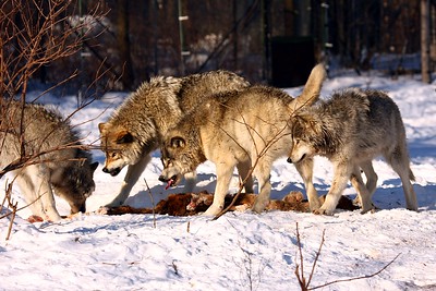
Every winter in Canada hunters shoot and trap wolves for their pelts. This hunting reduces the population size of wolves, but it has many other knock on consequences. For example, hunting also removes individuals from social groups which disrupts the wolf’s social hierarchy.
Questions about the world
Biologists have many questions about the impact of such hunting upon the wolves:
- Does hunting change a wolf pack’s behaviour?
- Do hunted wolves show signs of stress?
- Does hunting impact a wolf packs individual reproductive rate?
- Are all wolves affected equally by hunting?
And the list goes on.
We’ll focus on one question:
Do hunted wolves show signs of stress?
We happen to have a dataset that is relevant to this question: the WOLF.CSV data. This file contains data on individual wolves from three populations. Population 1 had almost no hunting intensity, population two had heavy hunting intensity and population 3 was a captive population. Cortisol concentrations from hair samples of individual wolves are also in this dataset. Cortisol is a physiological marker of stress.
To study this the above question we have:
- A response variable: Quantitative data on the main topic of interest (stress) in the form of individual cortisol concentrations (units of pg/mg).
- An explanatory variable: Data that might explain some of the variation in the response. In this case hunting intensity may help explain wolf stress levels. It is a qualitative variable (the population identity).
Hypotheses
We’re going to write our question as atestable statement, which is called a hypothesis. It is very important that this hypothesis is testable so that we can use our data to quantitatively test the hypothesis.
Start with a hypothesis about the effect of hunting on cortisol concentrations, which we’ll call thealternative hypothesis (H~1):
- H1: Wolves in population 2 (heavily hunted) have average cortisol levels that are higher than wolves in population 1 (almost not hunted).
We’ll also write a hypothesis that is a statement about no effect, which we’ll call thenull hypothesis (H0)
- H0: Wolves in population 2 have the same average cortisol levels as wolves in population 1
Testable predictions
If these hypotheses are fit for purpose we should be able to generate a testable prediction (or several predictions) from each hypothesis.
For example:
| Hypothesis | Prediction |
|---|---|
| H1 | Prediction 1: The concentration of cortisol in a sample of wolf hair from population 2 will be higher, on average, than a sample of hair from population 1. |
| H1 | Prediction 2: The concentration of cortisol in blood samples from population 2 will be higher, on average, than a sample of blood from population 1. |
| H0 | Prediction 1: On average, the concentration of cortisol in a sample of wolf hair from populations 1 and 2 will be the same. |
| H0 | Prediction 2: On average the concentration of cortisol in blood samples from populations 1 and 2 will be the same. |
Importing the data
First we import our data (our sample which gives partial infomration about our system). We make sure that the data type of thePopulationvariable is set as qualitative using the functionas.factor().
wolf = read.table('WOLF.CSV', header=T, sep=',')  # Import wolf data set
wolf$Population = as.factor(wolf$Population)      # Set Population as a qualitative variable
We will focus on populations 1 and 2 (light and heavy hunting respectively), so let’s subset our data to contain only these two populations.
wolf12 = droplevels(subset(wolf, Population!=3)) # Extract data from population 1 & 2Notice that we have used thedroplevels()function to ‘update’ the levels of the factors in thewolf12data frame. Thisdroplevels()function will force R to forget about the level for population 3.
Exploratory data analysis
After importing the data it’s important to start making a picture of the data by visualising the data using numerical and graphical summaries.
Numerical data exploration
First let’s look at a summary of the data
summary(wolf12) # Numerical summary of the data Individual Sex Population Colour
Min. : 1.00 Length:148 1: 45 Length:148
1st Qu.: 37.75 Class :character 2:103 Class :character
Median : 74.50 Mode :character Mode :character
Mean : 74.50
3rd Qu.:111.25
Max. :148.00
Cpgmg Tpgmg Ppgmg
Min. : 4.75 Min. : 3.250 Min. :12.76
1st Qu.:12.16 1st Qu.: 4.378 1st Qu.:19.50
Median :15.38 Median : 5.030 Median :25.00
Mean :16.61 Mean : 5.617 Mean :25.89
3rd Qu.:19.98 3rd Qu.: 6.067 3rd Qu.:30.01
Max. :40.43 Max. :15.130 Max. :53.28
NA's :79 Start to get a feeling for the numbers. Note the names of the variables, their range, the central tendency and their spread.
We can calculate the central tendency for each population using theaggregate()function
# Calculate mean Cortisol in each population
aggregate(Cpgmg~Population, data=wolf12, FUN=mean)
Population Cpgmg
1 1 15.56222
2 2 17.07495Notice that mean cortisol is higher in population 2. Is that the pattern we’d expect?
Graphical data exploration
Exploring the data with graphics is also useful
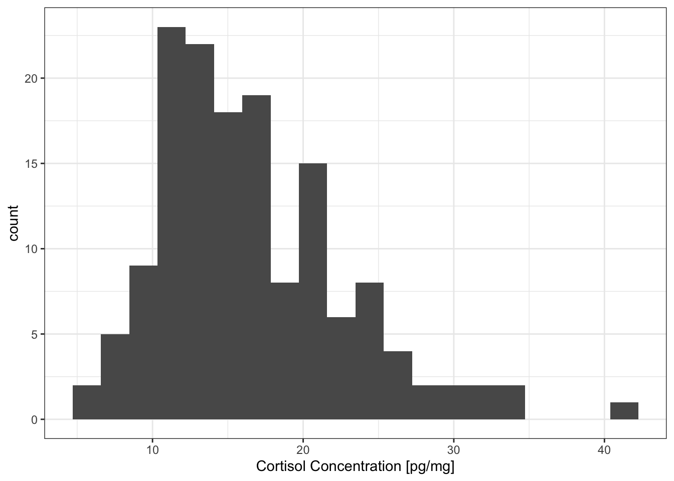
library(ggplot2) # Load ggplot2First we’ll look at thedistributionof the cortisol concentrations
# Plot the distribution of the cortisol data
ggplot(data=wolf12,
       aes(x=Cpgmg)) +
  geom_histogram(bins=20) +
  labs(x='Cortisol Concentration [pg/mg]') +
  theme_bw()
The distribution looks slightly right-skewed.
We can plot the raw data
# Plot the raw cortisol data
ggplot(data=wolf12,
       aes(x=Population,
           y=Cpgmg,
           colour=Population)) +
  geom_point(position='jitter') +
  labs(x='Population',
       y='Cortisol Concentration [pg/mg]') +
  theme_bw()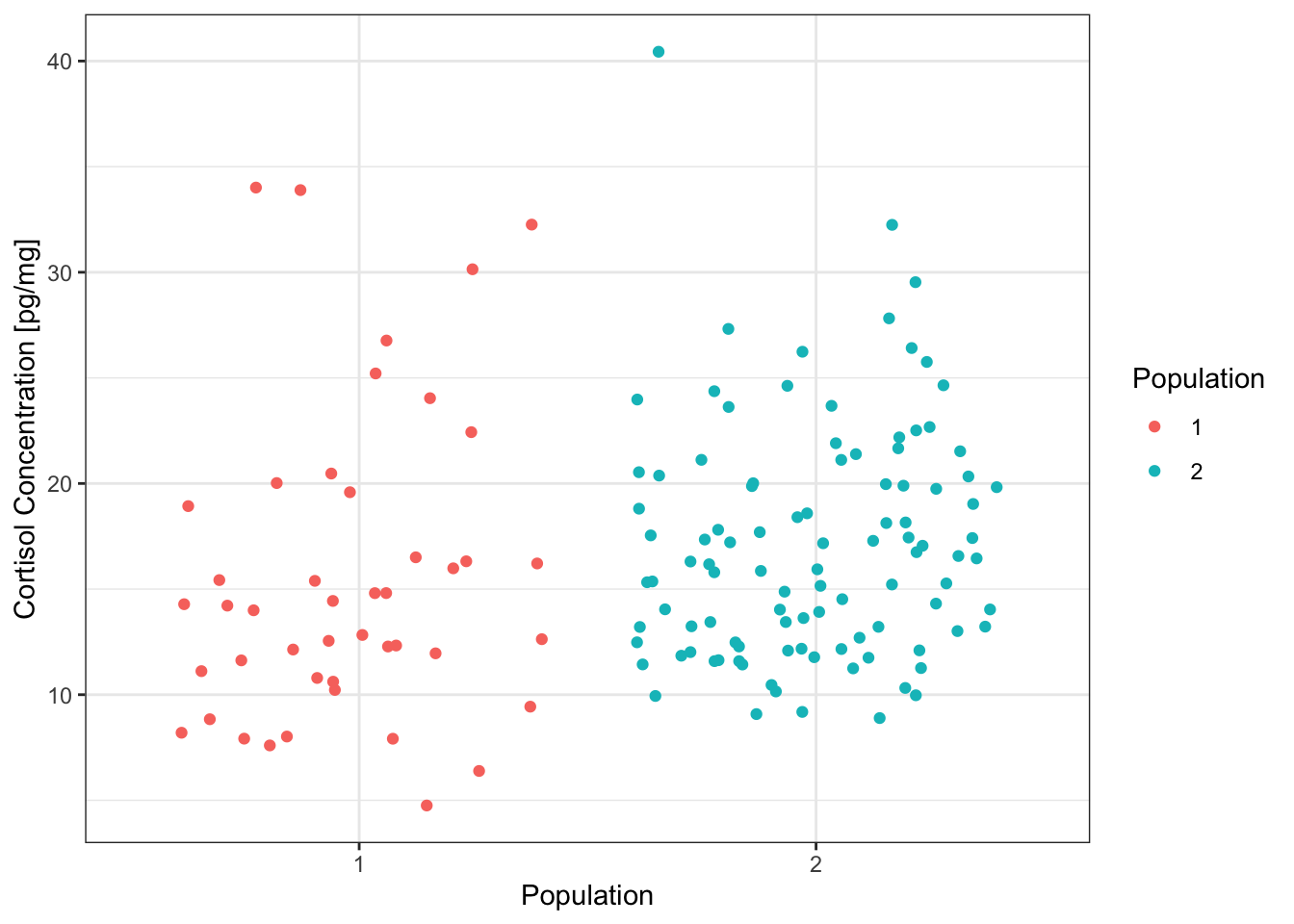
or summarise the data with a boxplot. Importantly, The boxplot not only visualises the central tendency of the data from the two populations (the median) but also the spread (in terms of the 25% and 75% quantiles as well as the whiskers).
# Draw a boxplot of the cortisol data from populations 1 and 2
ggplot(data=wolf12,
       aes(x=Population,
           y=Cpgmg)) +
  geom_boxplot() +
  labs(x='Population',
       y='Cortisol Concentration [pg/mg]') +
  theme_bw()

Median cortisol levels in population 2 are slightly higher than population 1, but there is a lot of spread about the central tendency.
A violin plot is an alternative to a boxplot
# Draw a violin plot of the cortisol data from populations 1 and 2
ggplot(data=wolf12,
       aes(x=Population,
           y=Cpgmg)) +
  geom_violin() +
  labs(x='Population',
       y='Cortisol Concentration [pg/mg]') +
  theme_bw()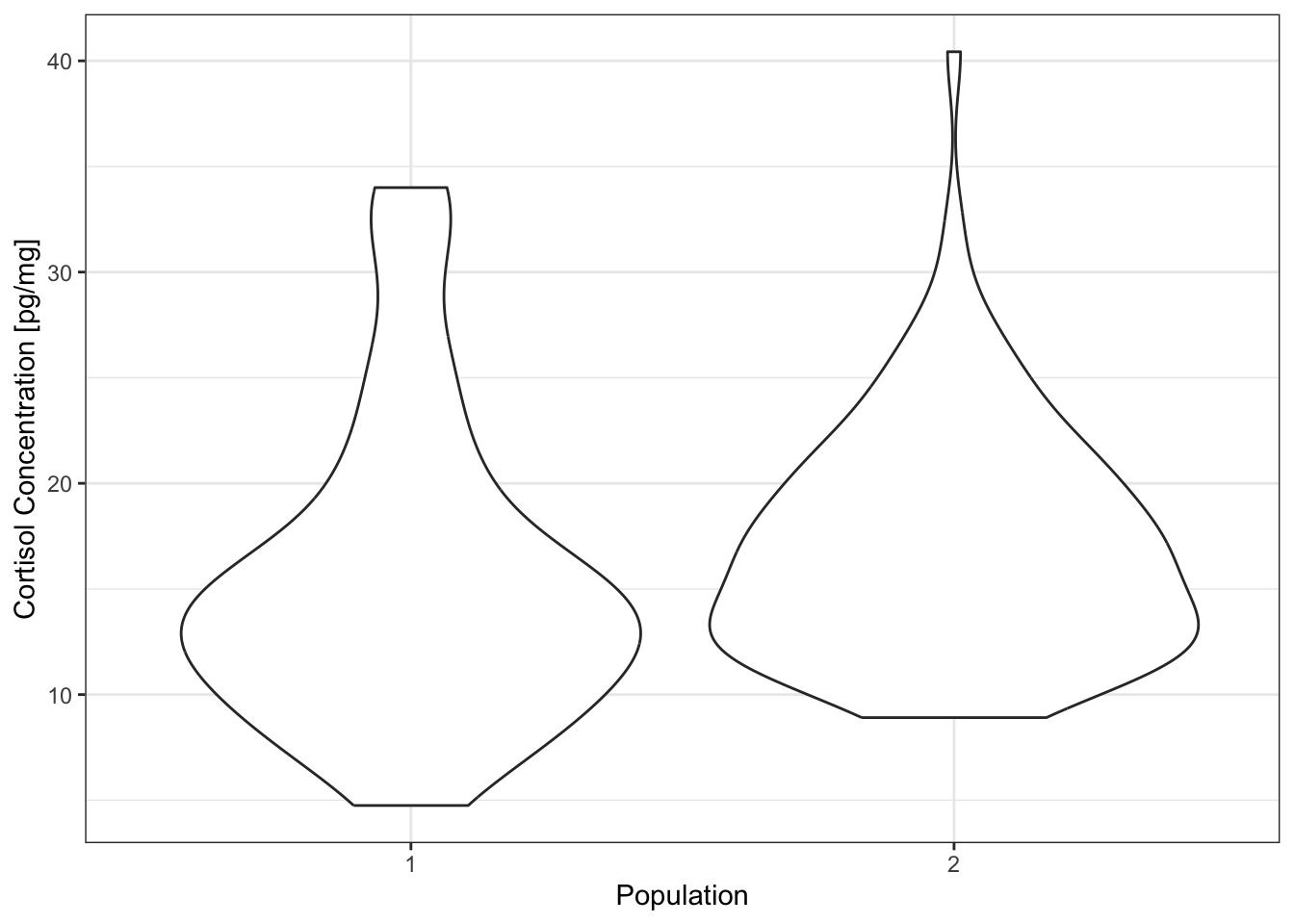
We may want to look at how several variables are able to explain cortisol values (the response variable). For example, differences between males and females and differences between the two populations.
# Draw a violin plot of the cortisol data from populations 1 and 2
# for males and females
ggplot(data=wolf12,
       aes(x=Population,
           y=Cpgmg,
           fill=Sex)) +
  geom_violin() +
  labs(x='Population',
       y='Cortisol Concentration [pg/mg]') +
  theme_bw()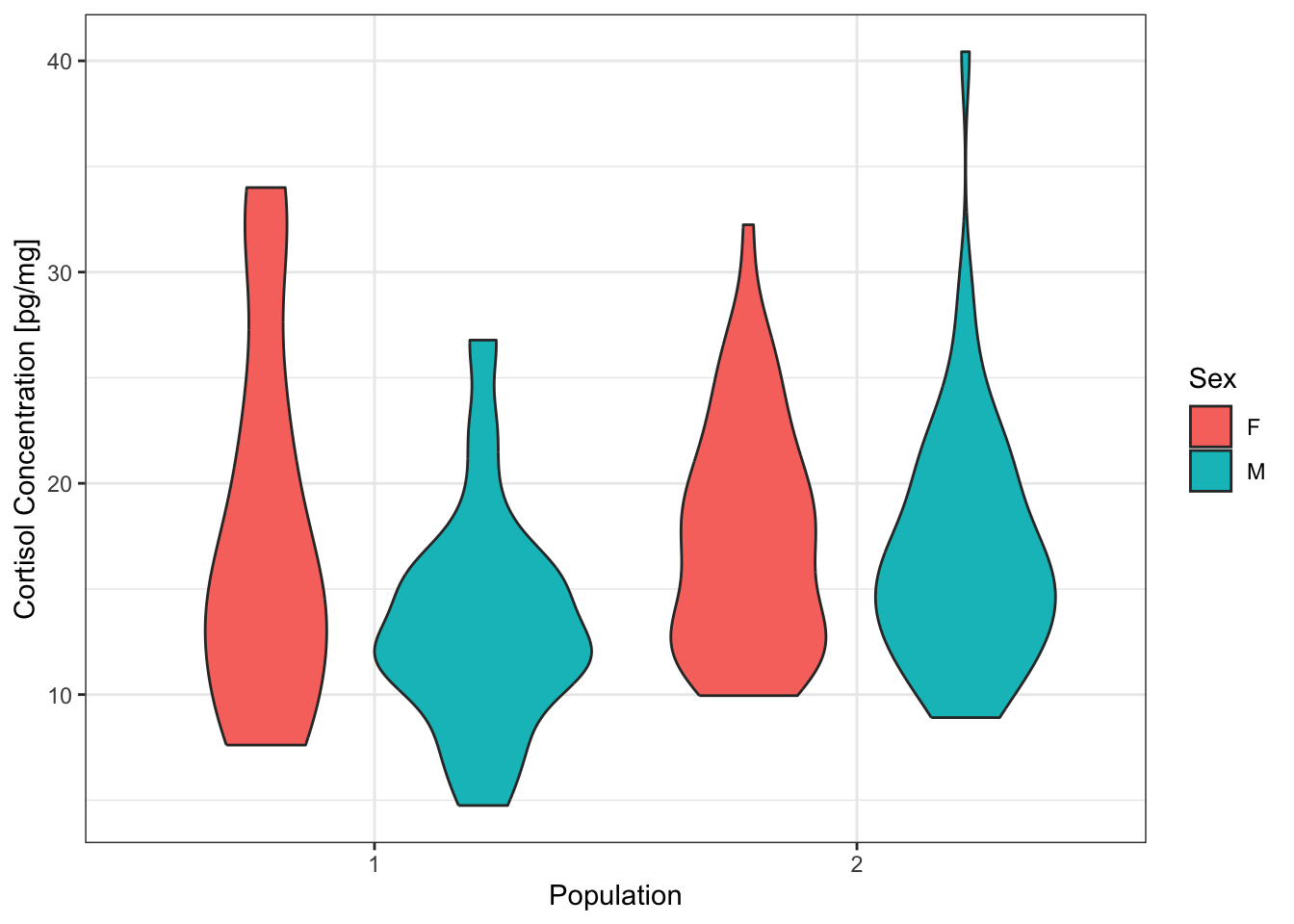
Balanced and unbalanced data
Use thetable()function to look at how much data we have from each population.
# Look at the balance of the data across
# levels of Population
table(wolf12$Population)
  1   2
 45 103
The sample size for population 1 is lower than population 2. This is called anunbalanced designand is very common when working with data collected from the field. Abalanced designis when sample sizes are the same for all levels of a factor. Classical ANOVA analysis required the data to be balanced. So these data would require special treatment if analysed with a classical ANOVA. General linear models can be used with unbalanced data, because they use maximum likelihood to fit the model. However, general linear model analysis is easiest for balanced data sets, and they should not be used for data that are extremely unbalanced.
Analyse the data
Modelling the population
Our data are asample. The data contain partial information about the topic of ourhypotheses(i.e. thepopulation). The population is the set of cortisol concentrations from all wolves from the two locations, at any time of the year, and maybe even across more of ta wolf’s body than just the hair.
If we are going to investigate our hypotheses then we need a way to describe the population. We will use a statistical model to describe the distribution of data we may expect across the whole population.
A statistical model
The figure below sketches out a possible statistical model. It sketches the distribution of cortisol for populations 1 and 2. The model has three important aspects:
- Theresponse variableis cortisol concentration (on the x-axis), and it is a quantitative variable
- The average value of cortisol in each population is described by a number (represented as and , whose value is as yet not known). In other words, the average value in each population has a unique value than can bedetermined.Given complete infomration about the population we could determine the value precisely.
- The variation of cortisol values in each population is being described by anormal distribution. The variation within a population is being described as beingrandombecause we are not trying to specify unique values of cortisol for every individual wolf. Instead we are describing all the possible outcomes of cortisol values by a normal distribution. There is an important differnce to the last point:Given complete infomration about the population we could not determine the precise value of a wolf’s cortisol value, but we can assign a probability to observing a cortisol concentration.
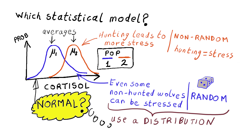
This model in the above sketch could be written in equation form as
Cpgmg=μi+Normal(0,σ)
where is the mean cortisol for population (is an index that can be 1 or 2) and is the standard deviation in cortisol values (i.e. the spread in cortisol values).
Note that:
- the spread is the same in both population 1 and 2.
- is shorthand for a normal distribution with meanof zero and standard deviation .
General linear models
The sketch above is a representation of a general linear model. General linear models are a hugely important family of statistical models.
A general linear model always uses a normal distribution to describe variation in the population that we will not try to associate with another variable (e.g. variation in cortisol concentrations between wolves in a population). The normal distribution in a general linear model is assumed to have a mean of zero and a constant standard deviation that must be estimated from data.
Special cases of general linear models are the methods of: linear regression, t-tests, analysis of variance (ANOVA) and analysis of covariance (ANCOVA).
General linear models are a statistical tool that allow us to:
- Analyse a very wide range of data with one statistical methodology
- Always describe randomness using a normal distribution
- Estimatemeans and other parameters of the population (e.g. the difference in mean cortisol between populations)
- Estimate the uncertaintyin population parameters from point 3.
- Quantify the strength of evidenceagainst the null-hypothesis
The work-horse function in R for fitting general linear models to data is thelm()function.
We will use the general linear model framework to estimate mean cortisol values in populations 1 & 2, and then test the hypothesis that these means are the same. We will then compare this approach to a t-test approach and finally to a permutation test approach.
Hypotheses revisited
Each hypothesis (the null-hypothesis, H0and the alternative hypothesis, H1) can be expressed in terms of our statistical model.
Model for H0
The null-hypothesis states that the there is no difference in average cortisol concentrations between populations 1 and 2.
This means that . The model corresponding to this is sketched below.
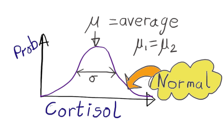
This model could also be written in equation form as
where is the mean cortisol in population 1 or 2 and is the standard deviation in cortisol values
In R the formula for this model is written simply asCpgmg ~ 1(for more details on how to specify a model using a formula go tohttp://www.ucd.ie/ecomodel/Resources/R_formulae_WebVersion.html).
You could also think of this model in terms of trying to predict average cortisol values. To predict average cortisol in either population 1 or population 2, given this null-hypothesis, you would make the same prediction () for both population.
Therandom part(represented by ) is always assumed to be a normal distribution when using thelm()function becauselm()fits a general linear model to the data. Thedeterministic part(sometimes called thesystematic part) in the formulaCpgmg ~ 1is represented by the1which means that it is a constant (i.e. there is one mean that is not affected by any other variable). This constant is called theInterceptby R.
Model for H1
The hypothesis states that average cortisol is different in populations 1 and 2.
This means that . The model corresponding to this is our first sketch showing two bell shaped normal distributions.
A sketch of the statistical model for the hypothesis H1
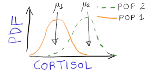
We therefore need two average values (and ) plus an estimate of spread () to specify the model for this hypothesis.
You could also think of this model in terms of trying to predict average cortisol values. To predict average cortisol in either population 1 or population 2, given this alternative-hypothesis, you would make the prediction for population 1 and for population 2 (i.e. different predictions.
In R the formula for this model will be written simply asCpgmg ~ 1 + Population
Formulas in R:Click here for more details on how to specify a model using a formula
Remember:
The random part of a general linear model is always assumed to be a normal distribution when using thelm()function.
The deterministic part now includes the factorPopulationto show that separate means should be fitted to population 1 and 2 (each level of the factor). The factorPopulationis an example of anexplantory variable.
Model parameters
- The model for H0has two parameters: and .
- The model for H1has three parameters: , and .
Parameters can also be calledcoefficients. The termcoefficientis commonly used when talking about the deterministic part of a model.
Fitting each of these models to thewolf12data involves estimating values for these parameters. Thelm()function fits each model using a method calledmaximum likelihood.
Fitting a model to data
Use thelm()function to fit a general linear model to data.
To use thelm()function we specify the model using aformula(see above) and specify the data frame containing the data.
Our formulas are
- H0model:
Cpgmg ~ 1 - H1model:
Cpgmg ~ 1 + Population
Theresponse(Cpgmg) is on the left hand side of the tilde (~) and thedeterministic partof the model (theexplanatory variables) is on the right hand side of the tilde. Therandom partis not represented in the formula because it is automatically taken to be a normal distribution. The functionlm()always assumes the random part of a model is a normal distribution.
Here is the R code to fit the H0model (null model) and the H1model (alternative model)
# Fit a linear model for the null-model
# (i.e. Population is not part of the model)
m0 = lm(Cpgmg ~ 1, data=wolf12)


# Fit a linear model for the alternative model
# (i.e. Population affects cortisol)
m1 = lm(Cpgmg ~ 1 + Population, data=wolf12)
Summarising the fitted model
Thesummary()function to can be used to view the fitted models.
summary(m0) # Summarise the null model
Call:
lm(formula = Cpgmg ~ 1, data = wolf12)

Residuals:
    Min      1Q  Median      3Q     Max
-11.865  -4.455  -1.240   3.360  23.815

Coefficients:
            Estimate Std. Error t value Pr(>|t|)
(Intercept)  16.6150     0.5051    32.9   <2e-16 ***
---
Signif. codes:  0 '***' 0.001 '**' 0.01 '*' 0.05 '.' 0.1 ' ' 1

Residual standard error: 6.145 on 147 degrees of freedom
The summary of each model prints:
Call:thelm()command used to fitted the modelResiduals:the quartiles of theresiduals(described in later tutorials)Coefficients:the fitted parameters for the deterministic part of the model (called the model coefficients) and their uncertainty (standard errors). For model m0 this is just the mean cortisol (called theIntercept) with an estimated value of 16.6 (standard error=0.51).Residual standard error:the fitted value for the standard deviation of the normal distribution in the statistical model. For the m0 model this issn-1= 6.14.- the residual degrees of freedom. This is the number of data points (=148) minus the number of parameters in the deterministic part of the model. For model m0 there is one parameter in the deterministic part of the model (), therefore the residual degrees of freedom = 147.
If the model is more complex than fitting a single mean (e.g. model m1) thensummary()also prints:
Multiple R-squared:the R2of the model. For model m1 the R2=0.013. The R2can be interpreted as the percentage of the variance in the response that is explained by the deterministic part of the model.- an adjusted R2which we will not be considering.
F statistic:an additional F statistic which we will not be considering
Interpreting model coefficients
Model H0
The H0model has one coefficient, the mean cortisol value, (output fromsummary(m0)). This is estimated to be 16.61 (s.e. 0.51). This information is from the(Intercept)row in the model summary info.
Remember:
that a fitted coefficients has anuncertaintybecause we used asampletoestimatea property of the population.It is important to give an uncertaintywith every estimated value from a model (a standard erroror a95% confidence interval).
We advise you to use a 95% confidence interval (confidence intervals will be discussed in a later tutorial):
- Use the
coef()function to quickly see the fitted values for a model’s coefficients - Use the
confint()command to obtain 95% confidence intervals in these fitted coefficients
# Model coefficient estimates and uncertainties

coef(m0)      # Coefficients for model m0
(Intercept)
16.615 confint(m0) # 95% confidence intervals on the coefficients for model m0 2.5 % 97.5 %
(Intercept) 15.61685 17.61315We can now report our estimate for the mean cortisol value (notice that we back transform to quote the result in the original units, not on the log-scale):
The average cortisol for all wolves from populations 1 and 2 is 16.61 pg/mg (95%CI: 15.62 - 17.61)
Model H1
The H1model has two coefficients:
coef(m1) # Coefficients for model m1(Intercept) Population2
15.562222 1.512729 confint(m1) # 95% confidence intervals on the coefficients for model m1 2.5 % 97.5 %
(Intercept) 13.7575212 17.366923
Population2 -0.6505745 3.676033- the mean cortisol value for population 1 (). This is estimated to be 15.56 (95% CI: (95% CI: 13.76 - 17.37). This is the coefficient labelled
(Intercept). - thedifferencebetween the means of population 1 and 2 (). Thisdifferenceis estimated to be 1.51 (95% CI: -0.65 - 3.68). This is the coefficient labelled
Population2.
Residuals
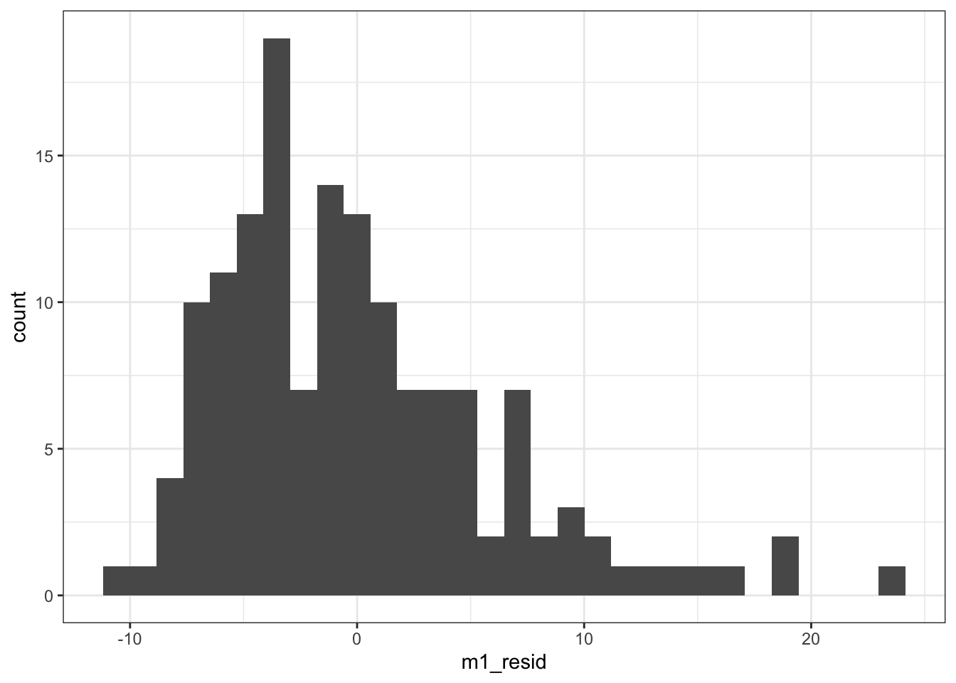
A residual is the difference between a data point and the prediction from a model. The residual is therefore associated with the random part of the model. It is the part of the response that cannot be explained by the model.
Most of the assumptions in our statistical model concern the residuals. So we will look at residuals in more detail when we discuss if the fitted model obeys the assumptions (model validation is the subject of a later tutorial).
The residuals of a fitted linear model can be obtained with theresiduals()function
m1_resid = residuals(m1) # Extract the residuals for model m1The distribution of residuals has a mean of zero,
mean(m1_resid) # Mean of the residuals from model m1[1] 5.521109e-16The calculated mean is extremely close to zero. It is not exactly zero because of the limited accuracy of the computer (remember1.0e-16is computer shorthand for 1x10-16= 0.0000000000000001).
The distribution of residuals can also be visualised by plotting a histogram
# Plot the distribution of residuals from model m1
ggplot(data=as.data.frame(m1_resid),
       aes(x=m1_resid)) +
  geom_histogram(bins=30) +
  theme_bw()
The standard deviation of the residuals is close to being an estimate of from our statistical model (it is a slight under-estimate).
sd(m1_resid) # Standard deviation of the residuals[1] 6.104729A more precise estimate is given by theresidual standard errorin thesummary()output.
Long-hand calculation of residuals
Residuals can be calculated explicitly by subtracting the model predictions (using thepredict()function) from the original data.
m1_resid2 = wolf12$logCpgmg - predict(m1) # Calculate residuals by handHave a go at comparing the two approaches for calculating residuals and show that they give the same answer
Summary of the topics covered
- The statistical model for general linear models revolves around the Normal distribution
- General linear models always use a normal distribution as the random part
- The variable of interest is called the response variable
- Statistical models of data always have a deterministic and a random part
- Statistical models have parameters
- The values of a model’s parameters can be estimated by fitting a model to data
- The
lm()function fits general linear models to data
Further Reading
All these books can be found in UCD’s library
- (opens in a new window)Cohen, J. (1990). Things I have learned (so far). American Psychologist, 45(12), 1304–1312.
- (opens in a new window)Cohen, J. (1994). The earth is round (p < .05). American Psychologist, 49(12), 997–1003.
- Andrew P. Beckerman and Owen L. Petchey, 2012Getting Started with R: An introduction for biologists(Oxford University Press, Oxford) [Chapter 5]
- Michael J. Crawley, 2015Statistics : an introduction using R(John Wiley & Sons, Chichester) [Chapters 7, 8]
- Tenko Raykov and George A Marcoulides, 2013Basic statistics: an introduction with R(Rowman and Littlefield, Plymouth)
